Crossing cells in Excel is quite simple, but with Google Sheets you do not have the option to cross cells and will need another application to support. There are several ways for us to cross cells in Google Sheets and these methods are relatively simple and easy to do. Below are instructions for crossing cells in Google Sheets.
How to Cross Out Cells in Google Sheets
Step 1:
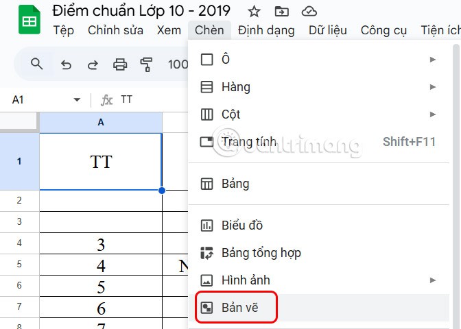
First, you enter the content into the Sheets cell , adjust the text to be opposite each other, use the line break shortcut in Google Sheets to enter the text. You click on the cell where you want to create a cross, then click Insert and then click Drawing in the displayed list.

Step 2:
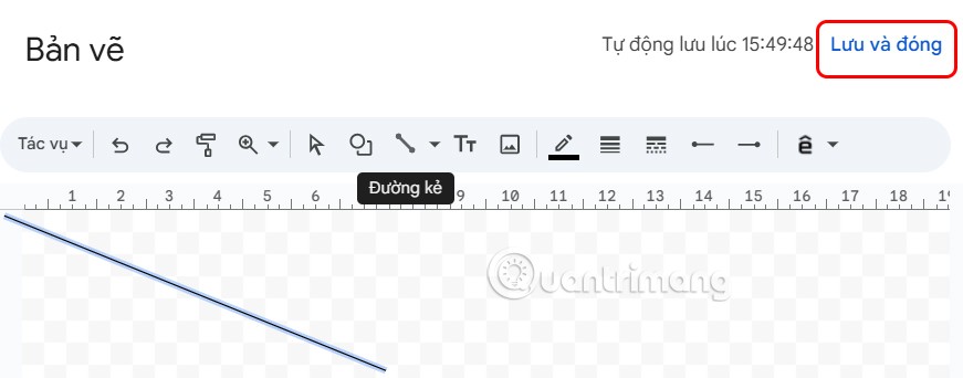
Display the drawing interface, select the Line icon as shown below.

Now you need to draw a line and then click Save and Close .

Step 3:
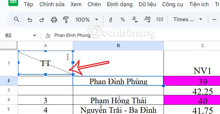
At this point, the user will see the line displayed in the cell and you need to adjust it to create a diagonal line in the Google Sheets cell . If you are not satisfied, click to edit it again.

As a result, we get a crossed-out cell in Google Sheets as shown.

How to create fake diagonal lines in Google Sheets
We will use the text rotation function to create a fake diagonal line in a Google Sheets cell.
Step 1:
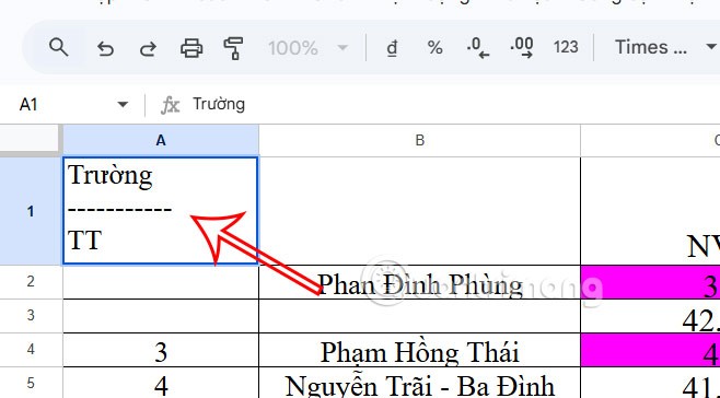
Type the first text in the cell and press ALT+Enter to create a new line. And type dashes to create a diagonal effect.
Step 2:
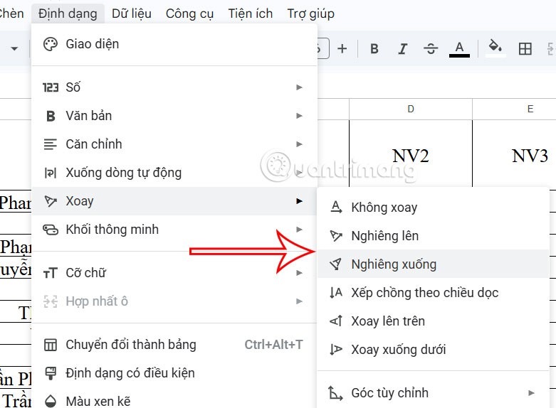
Click Format , then click Rotate and select the desired tilt angle .
