How to use VLOOKUP, INDEX, ... in Excel you should know

The functions VLOOKUP, INDEX, MATCH, ... are quite complex functions but are effective in data mining in Excel . In this article, I will guide you in detail how to use VLOOKUP and related functions effectively.

1. VLOOKUP function

Usage : Finds a specified value in the first column and pulls matching data from the same row in another column. This is one of the most popular functions and provides great support for complex office tasks.

Formula : = VLOOKUP (lookup_value, table_array, col_index_num, [range_lookup])

In which :

+ Lookup_value : The value to search.

+ Table_array : Two or more columns of data.

+ Col_index_num : Number of columns to pull data.

+ Range_lookup : Determine whether the search is completely accurate (FALSE) or just relatively accurate (TRUE or omitted).

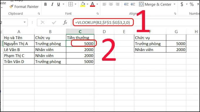
Example : We use the VLOOKUP function to find the Bonus of each employee. The value to look for is Cell Position C2; The array to detect is the array F1: G3. When entering the formula = VLOOKUP (C2, $ F $ 1: $ G $ 3,2,0) (1) the result is STAFF 2000 and ROOMER 5000 (2).

2. INDEX function

Usage : Returns a reference to a cell inside an array based on the number of rows and columns you specify.

Formula : = INDEX (array, row_num, [column_num])

Of which : Array (required): A cell range or an array constant.

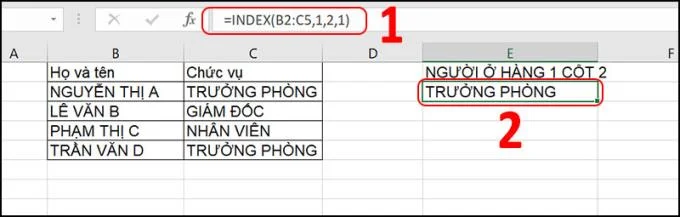
Example : When we need to get the value of the first row, second column in the table, we use the INDEX function . Array is the array we need to detect is B2: C5; Row_num is line 1; Column_num is column 2. When entering the formula INDEX (B2: C5,1,2,1) (1) the result is "HEAD OF ROOM" (2).

3. MATCH function

Usage : Looks up a specific value in a range of cells, and shows the relative position of that value.

Formula : = MATCH (lookup_value, lookup_array, [match_type])

In which :

+ lookup_value (required) : The value you want to match in the search array. Change the lookup value number can be a value (number, text, or logical value) or a cell reference to a number, text, or logical value.

+ lookup_array (required) : The range of cells to be searched.

+ match_type (optional) : Number -1, 0, or 1. The match type argument specifies how Excel matches the lookup value to values ​​in the lookup array. The default value for this argument is 1.

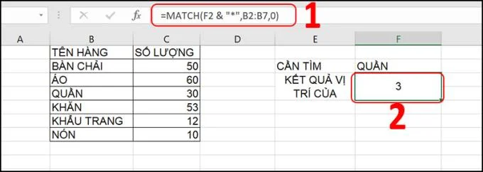
For example : When we need to know what position of CLOTH is in, we use MATCH function . When entering the formula = MATCH (FF2 & "*", "B2: B7", 0) (1), the result is 3 (2).

3. INDIRECT function

Usage : Returns a cell reference or range specified by a text string. Use the INDIRECT function when you want to change the reference to a cell in a formula without changing the formula itself.

Formula : = INDIRECT (ref_text, [a1])

In which :

+ Ref_text (required) : Reference to a cell containing the A1 reference style, the R1C1 reference style or a reference to the cell as a text string.

+ If the reference text is not a valid cell reference, INDIRECT returns the #REF! Error value . .

+ If ref_text refers to another workbook (an external reference), that workbook must be open. If the source workbook is not open, INDIRECT returns the #REF! Error value . .

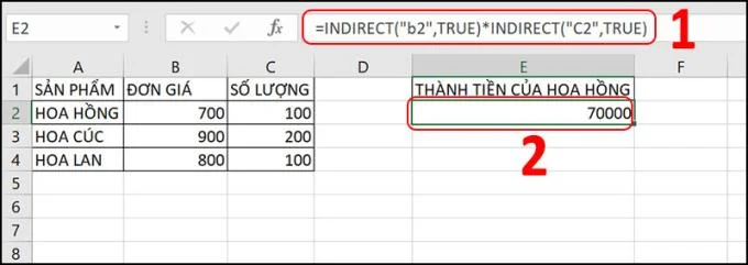
For example : When you only need to calculate the commission and you want to drag, drop or move the result box to another position without changing the money formula, we use INDIRECT . When entering the formula

= INDIRECT (“B2”, TRUE) * INDIRECT (“C2”, TRUE) (1) will give the result 700 * 100 = 70000 (2).

4. OFFSET function

Usage : Returns the reference to a range by a specified number of rows and a specified number of columns from a cell or range of cells. The returned reference can be a single cell or a range of cells. You can specify the number of rows and columns to return.

Formula : = OFFSET (reference, rows, cols, [height], [width])

In which :

+ Reference (required) : The reference area that you want to base the reference distance on. The reference range must refer to a cell or a range of adjacent cells; otherwise OFFSET returns the #VALUE! error value . .

+ Rows (required) : The number of rows, up or down, that you want the upper-left cell to refer to. Rows can be positive (which means below the starting reference) or negative (which means above the starting reference).

+ Cols (required) : Number of columns, to the left or right, that you want the cell in the upper left corner of the result to refer to. Columns can be positive or negative.

+ Height (optional) : The height, in number of rows, that you want to have for the returned reference. The height must be a positive number.

+ Width (optional) : The width, in the number of columns, that you want to have for the returned reference. Width must be a positive number.

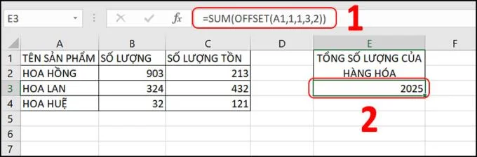
Example : We use OFFSET to localize values, and then use the SUM function to calculate the sum. The cell we refer to is A1; compared to A1, the Rows of the reference range is below 1 cell, so Rows is 1; compared to A1, the left Cols is 1 cell, so Cols is 1; Height we take 3 lines; Width we get 2 columns. So the result when adding up all the values ​​in the region is 2025.

5. TRANSPOSE function

Usage : Converts a horizontal range of cells into a vertical range and vice versa, i.e. converts rows into columns and columns to rows.

Formula : = TRANSPOSE (array)

Doing

+ Step 1 : Select blank cells.

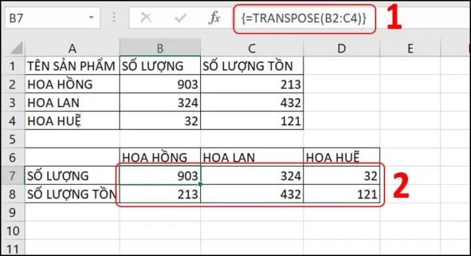
+ Step 2 : Enter = TRANSPOSE (B2: C4).

+ Step 3 : Enter the range of original cells.

+ Step 4 : Finally, press CTRL + SHIFT + ENTER.

Example : When we need to convert the whole product price list from vertical to horizontal, we use the TRANSPOSE function with the array of values ​​B2 to C4. When entering the formula = TRANSPOSE (B2: C4) (1) will give the result as shown (2).

6. HYPERLINK function

Uses : Creates a hyperlink to a document stored on the local network or the Internet.

Formula : = HYPERLINK (link_location, [friendly_name]).

In which :

Link_location can refer to a location in a document, like a specific cell or named range in a worksheet or in an Excel workbook, or to a bookmark in a Microsoft Word document.

The path can be to a file stored on the hard drive. The path can also be a universal naming convention (UNC) path on the server (in Microsoft Excel for Windows).

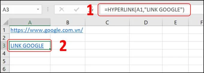
Example : Links that are long and confusing will be annoying to users. So please use HYPERLINK to make the interface easier to use. Entering the formula = HYPERLINK (A1, “LINK GOOGLE”) (1) will result in LINK GOOGLE (2).

The above article guided VLOOKUP and related functions. Hope that the above article will be useful to you.