How to Freeze, Hide Rows and Columns in Google Sheets

When working with Google Sheets, you will have to process dozens of columns of data. And if you make a mistake in processing because there are many columns, you should freeze the unused columns, or hide the columns or rows to make the Google Sheets table more compact.

Frozen or hidden columns or rows will no longer be visible or clickable. If we freeze the header row, it will be easier to read the document. In addition, there are many other options for freezing columns, in addition to freezing the first row or column. The following article will guide you on how to freeze, hide rows and columns in Google Sheets.

• Google Sheets Tricks You Shouldn't Miss
• How to edit chart notes in Google Sheets
• How to Add or Delete Rows and Columns in Google Sheets
• How to link data between spreadsheets in Google Sheets

Video tutorial on freezing, hiding columns and rows in Sheets

1. Freeze columns, rows in Google Sheets

Step 1:

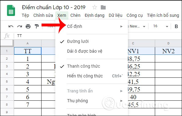
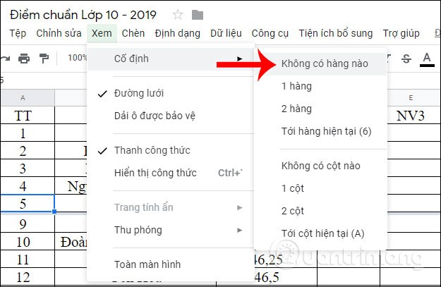
Click on the row or column you want to freeze, then click View and select Freeze .

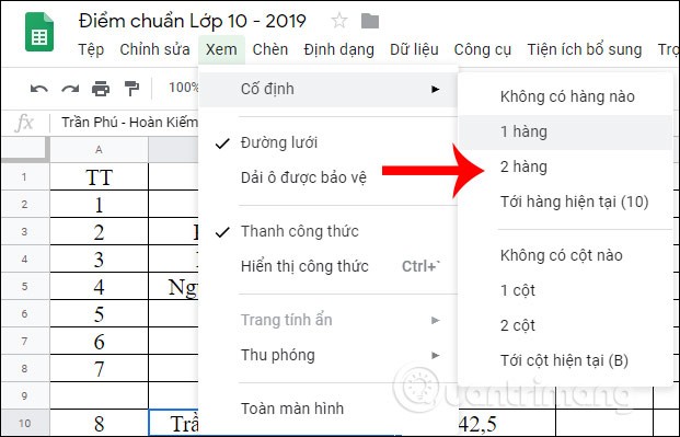
Now displays additional options for freezing columns and rows. If you click 1 row or 1 column, the first selected row and column will be frozen. If you click 2, the first 2 rows or 2 columns will be frozen.

Step 2:

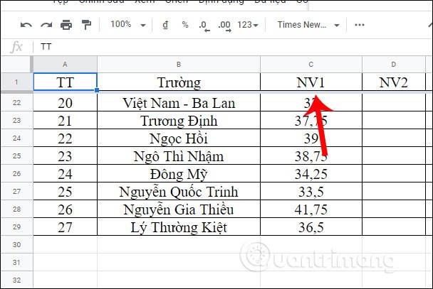
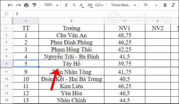
The row or column you selected is frozen. It is fixed with a gray border to separate it from the rest of the area, and cannot be moved no matter where you drag the mouse to.

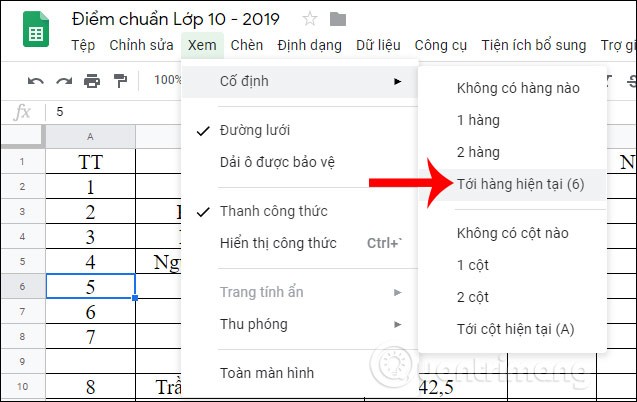
If the user wants to freeze an entire row or column , first click on the last cell in the row or column that needs to be frozen. Google Sheets will calculate from the first row or column down to the exact position you clicked. Then click View , select Freeze , then select Go to current row/column .

For example, to freeze from the first row to the 6th row, click on cell 5. At this point, Google Sheets calculates that there are 6 rows that need to be frozen.

The first 6 rows of results are fixed.

Step 3:

If you want to unfreeze a column or row , click View, select Freeze, then select No Rows (Columns) .

2. Hide columns and rows in Google Sheets

Step 1:

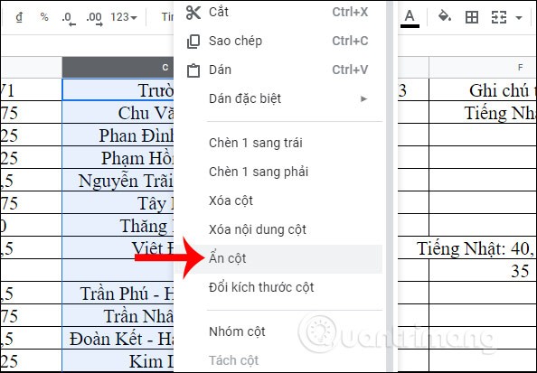
First click on the column header at the top then right click and select Hide column .

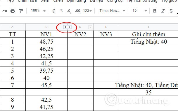
The selected column is now hidden and is symbolized by two arrows on both sides of the hidden column. If you click on this arrow icon , the column will automatically display .

Step 2:

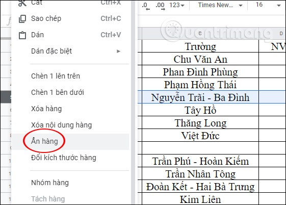
To hide rows in Google Sheets, users do the same, click on the first cell of the row and select Hide row .

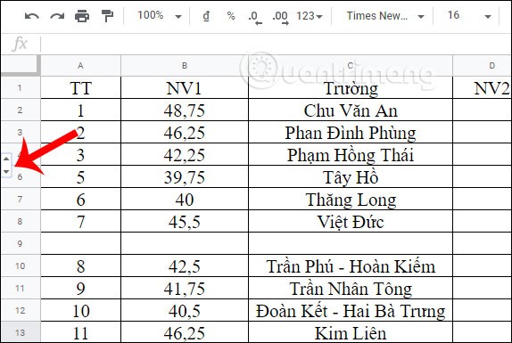
The result is that the row has been hidden and an arrow icon appears to indicate that the row has been hidden. To show the row again, just click on the arrow icon.

The operation of freezing rows, columns and hiding rows and columns in Google Sheets is very simple and easy to do. Once done, users cannot operate on locked or hidden areas, making it easier to tidy up the data table.

Good luck!