Instructions for naming Excel tables

By default, tables in Excel are named Table 1, Table2, Table 3,... but if you keep the names like this, it will be difficult to adjust and process the table. Therefore, users should change these fixed labels and name the Excel table, according to the instructions below.

How to name a table in Excel

Step 1:

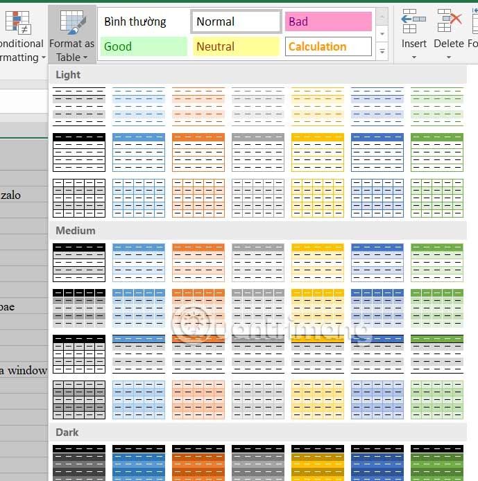
First you enter the data as usual, then click on any cell in the table and click Format As Table and choose the design that suits the data table.

You select the data area you want to draw a table and then click OK to execute.

Step 2:

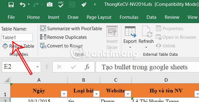
Continue clicking on the table and then click on Design and look down at the Properties group, you will see the Table Name item . Enter a new name for the table in this box.

If you want to rename the table later, select any cell in the table, click the Design tab, and then re-enter a different name for the Table Name.

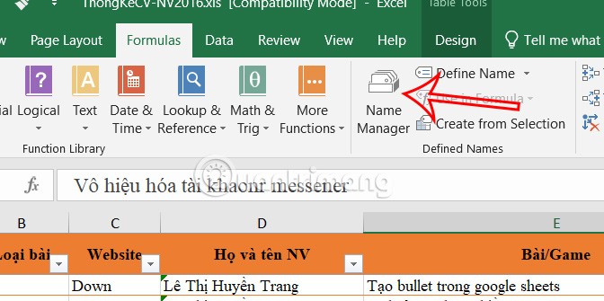
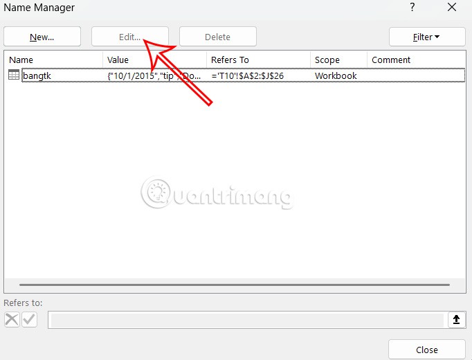
Or you click on the Formulas tab and then click on Name Manager to manage.

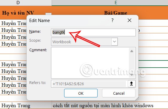
Now you will see the names of the data tables, click on the named table and click Edit below.

Finally, you enter a new name for the table.

Rules for naming tables in Excel

• Table names must begin with a letter, underscore (_), or forward slash (\).
• The remaining characters in the table name must be letters, numbers, periods, or underscores.
• A table cannot be named "C", "c", "R", or "r".
• Table names cannot be cell references, such as A1 or $B$2.
• Each table name in a spreadsheet must be unique.
• Keep your table names as short as possible and clearly identify the contents of the table. Table names can be up to 255 characters long.
• Table names cannot contain spaces. If a table name is made up of more than one word, use underscores or periods to separate the words.