How to use the FILTER function in Excel

If you regularly work with data sets in Excel, you know how important it is to be able to quickly find the information you need. Whether you're analyzing sales figures, tracking inventory, or managing a budget, the ability to filter data is essential.

Fortunately, Microsoft Excel has a powerful built-in tool that can help: the FILTER function. Using the FILTER function, you can quickly sort through large data sets and extract the data you need based on specified conditions.

Table of Contents

• What is the FILTER function?
• How to use the FILTER function in Excel
  • Using multiple criteria in the FILTER function
• How to use FILTER with other Excel functions
• Filter data effectively with Excel's FILTER function

What is the FILTER function?

The FILTER function in Excel allows you to extract a subset of data from a range based on one or more criteria. This function evaluates each value in a data range and returns rows or columns that meet the criteria you set. The criteria are expressed as formulas that evaluate to a logical value.

The FILTER function uses the following syntax:

=FILTER(array, include, [if_empty])

In there:

• array is the range of cells you want to filter.
• include represents the condition you want to use to filter your data. This can be a single criterion or multiple criteria separated by Excel logical functions.
• [if_empty] is an optional argument that specifies the return value if no data meets the specified condition.

How to use the FILTER function in Excel

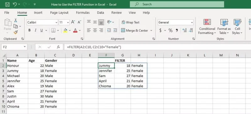
Let's look at an example to understand how to use the FILTER function in Excel. Suppose you have a data table that includes columns for Name, Age, and Gender, and you want to filter the table to show only females. You would use the following formula:

=FILTER(A2:C10, C2:C10="Female")

To parse the formula, the array argument is A2:C10 and the criteria argument is C2:C10="Female". This formula will return an array of values ​​that includes only rows where Gender is "Female".

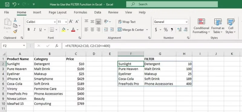
Let's look at another example! Let's say you have a data table that includes columns for Product Name, Category, and Price . You want to filter the table to show only rows with a price less than or equal to $400. You would use the following formula:

=FILTER(A2:C10, C2:C10<>

The FILTER function uses the logical operator (<=) to test the Price column for a condition that it is less than or equal to $400.

Using multiple criteria in the FILTER function

Excel's FILTER function allows you to specify more than one criteria to filter data. To add multiple criteria in the FILTER function, you need to use the "AND" or "OR" logical functions.

The AND function requires all criteria to be true for a row to be included in the filter results, while the OR function requires at least one of the criteria to be true for a row to be included in the results.

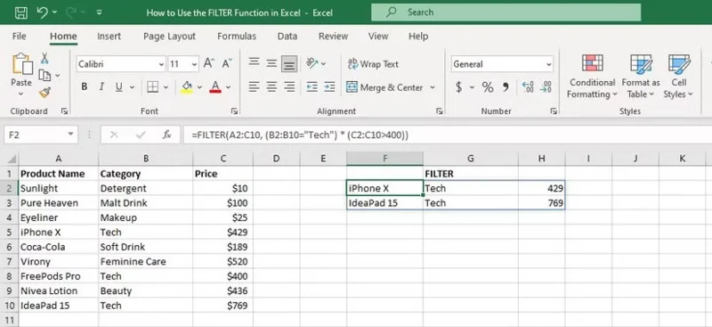
Here is an example of using the AND function within the FILTER function to extract data from a range based on two criteria:

=FILTER(A2:C10, (B2:B10="Tech")*(C2:C10>400))

This formula returns rows that meet two specified criteria. The first criterion is that the value in column B must be Tech and the second criterion is that the value in column C must be greater than 400 . The asterisk symbol ( * ) represents the AND operator, which combines the two criteria.

How to use FILTER with other Excel functions

The FILTER function in Excel can be used with many other functions to perform advanced calculations and analysis on specific sets of data in a large table.

A common way to use FILTER with other functions is to first filter a range of data with the FILTER function, and then apply another function to the filtered list. For example, you can sort data using the SORT function along with the FILTER function.

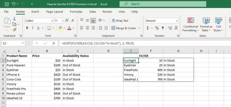
Here's an example: Suppose you have a table that contains information about different products including their names, prices, and availability. You want to filter the table to show only the products that are in stock and sort the filtered list by price.

The formula, in this case, would be:

=SORT(FILTER(A2:C10, C2:C10="In Stock"), 2, TRUE)

This formula will return a filtered table with only the products currently in stock, sorted by their price in ascending order. The second argument in the SORT function (i.e. 2) represents the column number you want to sort by.

In this case, we want to sort by the price in column B, so we use the number 2. The third argument in the SORT function (i.e. TRUE) specifies that we want to sort the values ​​in ascending order.

Here are other Excel functions that you can combine with the FILTER function:

• SUMIF or AVERAGEIF : You can use the FILTER function to create a subset of data that meets certain criteria, and then use the SUMIF or AVERAGEIF function to calculate the sum or average of that subset of data.
  • For example, if you have a list of sales data for different products and want to calculate the total sales for a specific product, you can use FILTER to create a subset of data for that product, and then use the SUMIF function to calculate the total sales.
• MAX and MIN : You can use the FILTER function to find the largest or smallest value in a subset of data that meets certain criteria. In the sales data example, you could use the FILTER function with MAX or MIN to find the product with the highest or lowest sales.
• COUNT : You can also use the COUNT function with FILTER to get the number of cells that meet certain criteria.

Overall, combining the FILTER function with other Excel functions can help you perform more advanced analysis and make your data more meaningful and useful.

Filter data effectively with Excel's FILTER function

Excel's FILTER function allows you to quickly and easily filter data based on specified conditions. Using the FILTER function, you can avoid the hassle of manually sorting through large data sets to find the data you need. You can specify multiple criteria and combine them using operators like "AND" and "OR", giving you flexibility and control over your filter formula.

Whether you're an experienced analyst or a beginner, Excel's FILTER function can help you streamline your workflow and get the most out of your data.